An Introduction to Planetary Computer – Visualize IPCC CMIP6 Geospatial Data

What is Planetary Computer?

The Planetary Computer from Microsoft launched as a market competitor of Google Earth Engine to support sustainable decision making with the power of their cloud technologies. The computational power is one of the biggest challenge of working with large-scale geospatial datasets of environment to make a decision at global scale. The cloud computing together with AI technologies solves the complex problem of our earth fetching now.

The Planetary Computer includes petabytes of global environmental datasets such as Landsat, Sentinel, ASTER, ALOS, GOES-R, NAIP, IPCC CMIP6, and so on which is continuously increasing day to day. All of this public datasets are easily accessible with their intuitive STAC API. The API let’s their user to find and discover the data by simplifying the searching and querying across their data catalog. The Planetary Computer provides an integrated Jupyter Notebook development environment called Planetary Computer Hubs to scale the analysis of complex large geospatial datasets with their cloud computing power. They also provides an applications that built on top of the Planetary Computer Platform.

In this tutorial, I will show you how to access the global NASA NEX-GDDP-CMIP6 data, visualize this data in Planetary Computer Hub.

About Datasets

The NEX-GDDP-CMIP6 dataset offers global downscaled climate scenarios derived from the General Circulation Model (GCM) runs conducted under the Coupled Model Intercomparison Project Phase 6 (CMIP6) and across two of the four “Tier 1” greenhouse gas emissions scenarios known as Shared Socioeconomic Pathways (SSPs). The purpose of this dataset is to provide a set of global, high resolution, bias-corrected climate change projections that can be used to evaluate climate change impacts on processes that are sensitive to finer-scale climate gradients and the effects of local topography on climate conditions.

Step – 1: Import the required libraries

import planetary_computer
import xarray as xr
import fsspec
import pystac_client

Step – 2: Access the Planetary Computer data catalog using pystac-client

catalog = pystac_client.Client.open(
 "https://planetarycomputer.microsoft.com/api/stac/v1",
 modifier=planetary_computer.sign_inplace,
)

Step – 3: Get CMIP6 datasets from data catalog

collection = catalog.get_collection("nasa-nex-gddp-cmip6")

Step – 4: List all of CMIP6 models

collection.summaries.get_list("cmip6:model")

There are 35 models available in the CMIP6 data.

['ACCESS-CM2',
 'ACCESS-ESM1-5',
 'BCC-CSM2-MR',
 'CESM2',
 'CESM2-WACCM',
 'CMCC-CM2-SR5',
 'CMCC-ESM2',
 'CNRM-CM6-1',
 'CNRM-ESM2-1',
 'CanESM5',
 'EC-Earth3',
 'EC-Earth3-Veg-LR',
 'FGOALS-g3',
 'GFDL-CM4',
 'GFDL-CM4_gr2',
 'GFDL-ESM4',
 'GISS-E2-1-G',
 'HadGEM3-GC31-LL',
 'HadGEM3-GC31-MM',
 'IITM-ESM',
 'INM-CM4-8',
 'INM-CM5-0',
 'IPSL-CM6A-LR',
 'KACE-1-0-G',
 'KIOST-ESM',
 'MIROC-ES2L',
 'MIROC6',
 'MPI-ESM1-2-HR',
 'MPI-ESM1-2-LR',
 'MRI-ESM2-0',
 'NESM3',
 'NorESM2-LM',
 'NorESM2-MM',
 'TaiESM1',
 'UKESM1-0-LL']

Step – 4: Get the scenarios

The CMIP6 datasets is composed of various scenarios.

collection.summaries.get_list("cmip6:scenario")

['historical', 'ssp245', 'ssp585']

The "historical" scenario covers the years 1950 - 2014 (inclusive). The "ssp245" and "ssp585" cover the years 2015 - 2100 (inclusive).

Step – 5: Get the variables

collection.summaries.get_list("cmip6:variable")

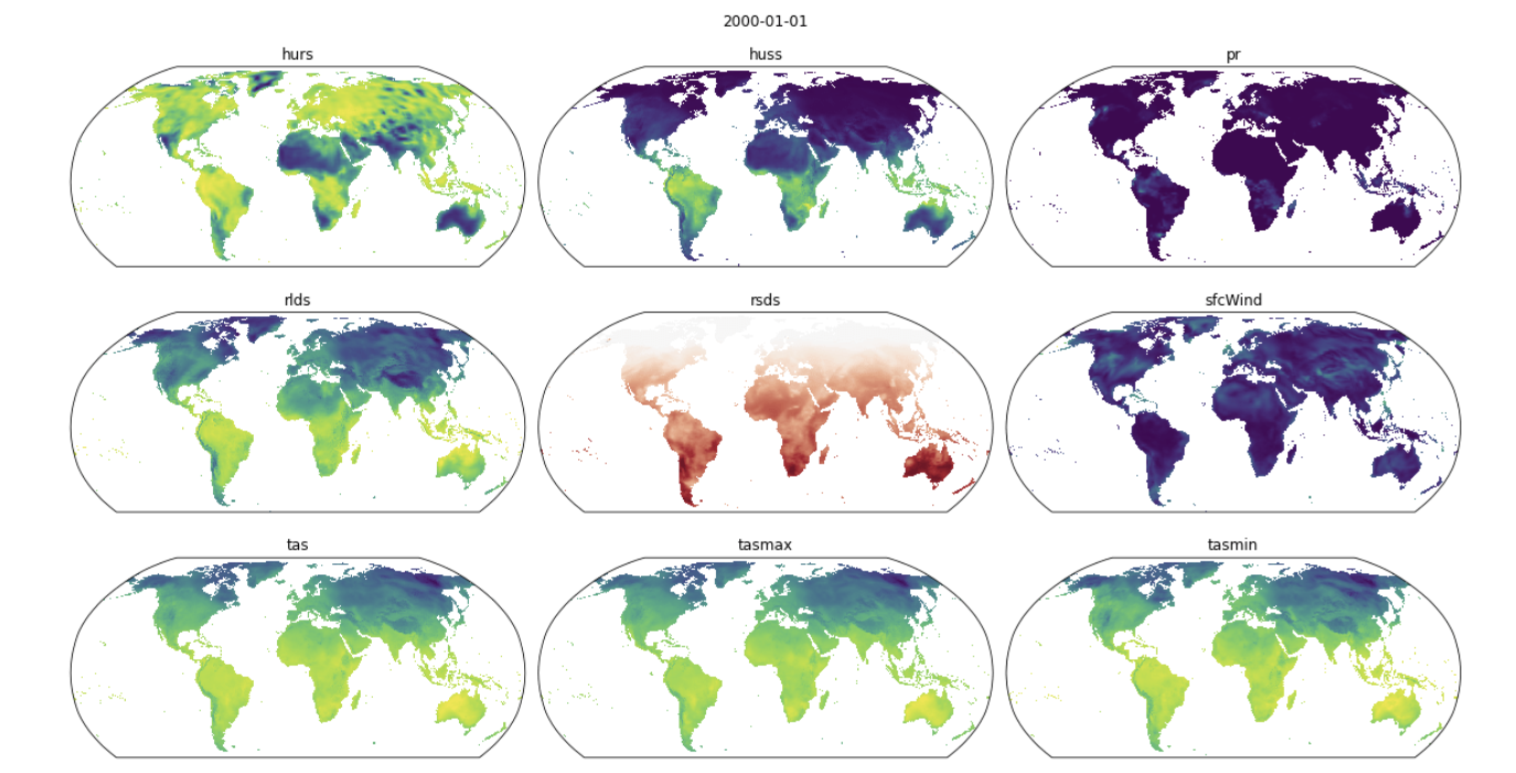
['hurs', 'huss', 'pr', 'rlds', 'rsds', 'sfcWind', 'tas', 'tasmax', 'tasmin']

Step – 6: Get specific data

search = catalog.search(
 collections=["nasa-nex-gddp-cmip6"],
 datetime="2022",
 query={"cmip6:model": {"eq": 'ACCESS-CM2'}},
)

items = search.get_all_items()
len(items)

Step – 7: List of assets in a item

item = items[0]
list(item.assets)

Step – 8: Read data in xarray

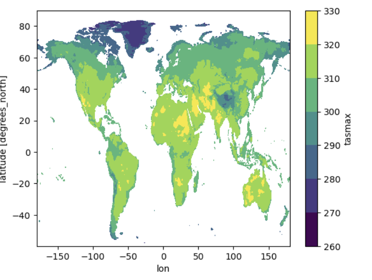
df = xr.open_dataset(fsspec.open(item.assets["tasmax"].href).open())

Step – 9: Convert the longitude from 360 to 180

df.coords['lon'] = (df.coords['lon'] + 180) % 360 - 180
df = df.sortby(df.lon)

Step - 10: Plot and visualize data

df.tasmax.plot.contourf()

Share To