Visualize NDVI in Microsoft Planetary Computer

What is Normalized Difference Vegetation Index (NDVI)?

The Normalized Difference Vegetation Index (NDVI) is quantify the vegetation by measuring the difference between near-infrared and red bands.

NDVI = (NIR-Red)/(NIR+Red)

NDVI value ranges between 1 to +1. The positive value tends to dense vegetation and negative value represents non-vegetation like water-bodies, snow etc.

In this tutorial, I will show you how to create an NDVI map from Landsat data in Microsoft Planetary Computer.

Step – 1: Environment setup

import pystac_client
import planetary_computer
import odc.stac
import matplotlib.pyplot as plt
from pystac.extensions.eo import EOExtension as eo

Step – 2: Access to Planetary Computer Data

catalog = pystac_client.Client.open(
    "https://planetarycomputer.microsoft.com/api/stac/v1",
    modifier=planetary_computer.sign_inplace,
)

Step – 3: Choose an area and time of interest

bbox_of_interest = [89.419391,22.732522,89.671905,22.853430] # Bounding box of study 
time_of_interest = "2022-01-01/2022-12-31" # Define start and end date

Step – 4: Define search parameters

search = catalog.search(
    collections=["landsat-c2-l2"],
    bbox=bbox_of_interest,
    datetime=time_of_interest,
    query={"eo:cloud_cover": {"lt": 1}},
)

Here, collections indicates the dataset, query to define cloud cover of image. The “lt” means less than. We set the cloud cover less than 1% means it will return the image collection where each image have less than 1% cloudy.

Step – 5: Identify the length of image collection

items = search.item_collection()
print(f"Returned {len(items)} Items")

Returned 25 Items

selected_item = items[5] # min(items, key=lambda item: eo.ext(item).cloud_cover)
print(
    f"Choosing {selected_item.id} from {selected_item.datetime.date()}"
    + f" with {selected_item.properties['eo:cloud_cover']}% cloud cover"
)

We randomly select the image which index number is 5. The print options shows the image id, date of acquisition and its cloud cover.

Choosing LC09_L2SP_138044_20221114_02_T1 from 2022-11-14 with 0.05% cloud cover

Step – 6: Exploring image bands

max_key_length = len(max(selected_item.assets, key=len))
for key, asset in selected_item.assets.items():
    print(f"{key.rjust(max_key_length)}: {asset.title}")

              qa: Surface Temperature Quality Assessment Band
             ang: Angle Coefficients File
             red: Red Band
            blue: Blue Band
            drad: Downwelled Radiance Band
            emis: Emissivity Band
            emsd: Emissivity Standard Deviation Band
            trad: Thermal Radiance Band
            urad: Upwelled Radiance Band
           atran: Atmospheric Transmittance Band
           cdist: Cloud Distance Band
           green: Green Band
           nir08: Near Infrared Band 0.8
          lwir11: Surface Temperature Band
          swir16: Short-wave Infrared Band 1.6
          swir22: Short-wave Infrared Band 2.2
         coastal: Coastal/Aerosol Band
         mtl.txt: Product Metadata File (txt)
         mtl.xml: Product Metadata File (xml)
        mtl.json: Product Metadata File (json)
        qa_pixel: Pixel Quality Assessment Band
       qa_radsat: Radiometric Saturation and Terrain Occlusion Quality Assessment Band
      qa_aerosol: Aerosol Quality Assessment Band
        tilejson: TileJSON with default rendering
rendered_preview: Rendered preview

Step - 7: Band selection

bands_of_interest = ["nir08", "red", "green", "blue", "qa_pixel"]
data = odc.stac.stac_load(
    [selected_item], bands=bands_of_interest, bbox=bbox_of_interest
).isel(time=0)
data

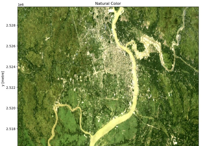
Step - 8: Plot and visualize the raw image

fig, ax = plt.subplots(figsize=(10, 10)) // Define plot size

data[["red", "green", "blue"]].to_array().plot.imshow(robust=True, ax=ax)
ax.set_title("Natural Color");

Step – 9: Calculate and visualize NDVI

red = data["red"].astype("float")
nir = data["nir08"].astype("float")
ndvi = (nir - red) / (nir + red)

fig, ax = plt.subplots(figsize=(10, 6))
ndvi.plot.imshow(ax=ax, cmap="viridis")
ax.set_title("NDVI");

GitHub Source Code Link - NDVI Planetary Computer

If you like this tutorial, please share with your connections . 

Share To