Visualize netCDF4 data in Python

What is a NetCDF4 file?

The Network Common Data Form (NetCDF) is a file format for storing multi-dimensional data such as temperature, humidity, pressure, wind speed, and direction. It is a highly flexible data format that can read metadata as an array. It was developed by UCAR and maintains standards and software that support the use of the format. The netCDF4 data standard is used broadly by the climate science community to store climate data. Climate data are -

• Time series data (daily, monthly and years=ly of historic or future projected data)

• Spatially distributed covering regions such as the United States or even the world.

• Model-driven which requires documentation making the self-describing an aspect of NetCDF files useful.

The NetCDF4 format store climate data in an array format. Climate data typically have three dimensions—x and y values representing latitude and longitude location for a point or a grid cell location on the earth’s surface and time. The arrays contain time-series data as time together with its spatial location as latitude and longitude.

In this tutorial, I will discuss reading, plotting, and mapping NetCDF4 formatted data in python using Jupyter Notebook. I will use NASA NEX-GDDP-CMIP6 maximum temperature data.

Open your Jupyter Notebook and Install the package.

Step -1: Install required packages

pip install netCDF4
pip install matplotlib

Step – 2: Import packages

import netCDF4
import matplotlib.pyplot as plt

Step – 3: Define data file path

file_path = "data/tasmax_day_GFDL-CM4_ssp245_r1i1p1f1_gr1_2022.nc"

Step – 4: Read data using netCDF4 python lib

nc = netCDF4.Dataset(file_path, mode="r")
print(nc)

<class 'netCDF4._netCDF4.Dataset'>
root group (NETCDF4_CLASSIC data model, file format HDF5):
    activity: NEX-GDDP-CMIP6
    contact: Dr. Rama Nemani: rama.nemani@nasa.gov, Dr. Bridget Thrasher: bridget@climateanalyticsgroup.org
    Conventions: CF-1.7
    creation_date: 2021-10-06T08:10:23.629541+00:00
    frequency: day
    institution: NASA Earth Exchange, NASA Ames Research Center, Moffett Field, CA 94035
    variant_label: r1i1p1f1
    product: output
    realm: atmos
    source: BCSD
    scenario: ssp245
    references: BCSD method: Thrasher et al., 2012, Hydrol. Earth Syst. Sci.,16, 3309-3314. Ref period obs: latest version of the Princeton Global Meteorological Forcings (http://hydrology.princeton.edu/data.php), based on Sheffield et al., 2006, J. Climate, 19 (13), 3088-3111.
    version: 1.0
    tracking_id: b007f79e-0905-46f5-b0d4-6118cd818cde
    title: GFDL-CM4, r1i1p1f1, ssp245, global downscaled CMIP6 climate projection data
    resolution_id: 0.25 degree
    history: 2021-10-06T08:10:23.629541+00:00: install global attributes
    disclaimer: This data is considered provisional and subject to change. This data is provided as is without any warranty of any kind, either express or implied, arising by law or otherwise, including but not limited to warranties of completeness, non-infringement, accuracy, merchantability, or fitness for a particular purpose. The user assumes all risk associated with the use of, or inability to use, this data.
    external_variables: areacella
    cmip6_source_id: GFDL-CM4
    cmip6_institution_id: NOAA-GFDL
    cmip6_license: CC-BY-SA 4.0
    dimensions(sizes): time(365), lat(600), lon(1440)
    variables(dimensions): float64 time(time), float32 tasmax(time, lat, lon), float64 lat(lat), float64 lon(lon)
    groups: 

Step – 4: Check the data type

print(type(nc))

Step – 6: Explore the variables

print(nc.variables.keys())

dict_keys(['time', 'tasmax', 'lat', 'lon'])

Step – 7: Explore specific variable

print(nc["tasmax"])

<class 'netCDF4._netCDF4.Variable'>
float32 tasmax(time, lat, lon)
    _FillValue: 1e+20
    standard_name: air_temperature
    long_name: Daily Maximum Near-Surface Air Temperature
    units: K
    cell_methods: area: mean time: maximum
    cell_measures: area: areacella
    interp_method: conserve_order2
    original_name: tasmax
    missing_value: 1e+20
unlimited dimensions: time
current shape = (365, 600, 1440)
filling on

Step - 8: Plotting data using matplotlib

plt.contourf(nc['tasmax'][0,:,:])
plt.colorbar()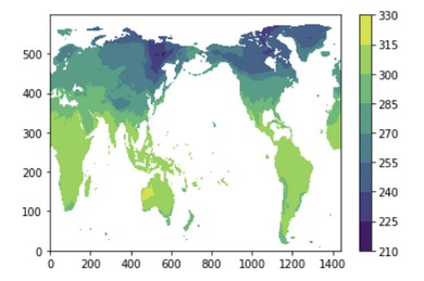

Step – 9: Change the default colormap

plt.contourf(nc['tasmax'][0,:,:], cmap='jet')
plt.colorbar()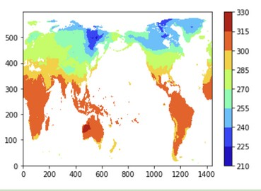

Matplotlib have different sets of the colormap. You can explore various colormaps here

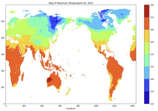
Step - 10: Change the figure size, add label and title of the figure

# Define figure size
plt.figure(figsize=(16,10))

# Add label and titile of figure
plt.xlabel("Longitude")
plt.ylabel("Latitude")
plt.title("Map of Maximum Temperature (K), 2022")

plt.contourf(nc['tasmax'][0,:,:], cmap='jet')
plt.colorbar()

Step – 11: Explore units of the temperature data

print(nc['tasmax'].units)

GitHub Source Code Link - Visualize NetCDF4 Data in Python

Share To